
Solving the Complex RBD-Series Parallel System with a Keystone Component
The general form of this type of reliability block diagram has two series circuits in a parallel arrangement combined through a center or “keystone” unit. You are often given the reliability of each block and asked to calculate the reliability of the circuit.
For example let’s say we are given the following five block arrangement pictured in Figure 1. Each of the blocks is identical and each has a failure rate of 10 failures per million hours (FPMH). For a 1,000 hour mission, what is the reliability of the circuit?
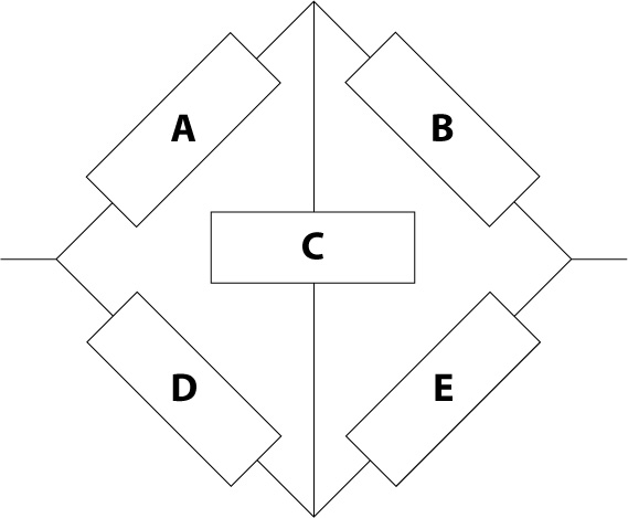
Figure 1 – Five Element RBD
The most commonly used method of solving this problem is by way of using a Bayesian approach. According to Bayes Theorem, the probability that the system is working (reliability) can be summed up from two components; first, the reliability of the system when Block C is functioning properly multiplied by the probability that C is working properly, and; second, the reliability of the system when C is not functioning properly multiplied by the probability that C is not working properly.
Mathmatically:
RSystem = RSystemC working * Probability C working + RSystem C failed * Probability C failed
Figures 2 and 3 show the block diagrams of the two scenarios:
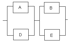
Figure 2 – Scenario A: |
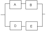
Figure 3 – Scenario B: |
Based on these two scenarios, the following equation expresses the system reliability:
Rs = C * ( ( A + D – AD ) * ( B + E – BE ) ) + ( 1 – C ) * ( AB + DE – ABDE )
We begin by calculating the reliability of Scenario A. Since each block in parallel circuit AD and BE is identical we can use the Redundancy Calculator tool in QuART PRO, as seen in Figure 4. Using a failure rate of 10FPMH and 1000 hours, we get a reliability of 99.99% for each. Since the product of these two parallel groups reflects the circuit when C is functioning, we then multiply this product by the reliability of Block C.
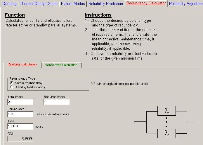
Figure 4 – QuART PRO Redundancy Calculator
We can do the same for Scenario B (the parallel arrangements of AB and DE). The result is then multiplied by the probability that C is in the failed state, 1 – Reliability of C.
Combining the two results yields a System reliability of 97.85%
Had the blocks not been identical, we could have just as easily used the Failure Rate calculator in QuART PRO, as seen in Figure 5, to calculate the failure rate for the two scenarios. Given the stated mission time, we can translate this failure rate to a system reliability number.
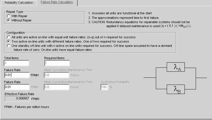
Figure 5 – QuART PRO Failure Rate Calculator
Another approach is to use a technique familiar with Fault Tree practitioners, the “cut-set” method. Here you simply examine the circuit in terms of all the combinations that would result in system failure.
If we look at the original circuit we notice that there are four block combinations that can cause the system to fail. These are AD, BE, ACE, and BCD. These four “cut-sets” are shown in Figure 6.
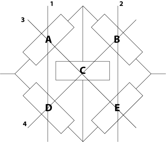
Figure 6 – Original Circuit Cut-Sets
We then generate a list of all possible combinations for the five blocks in the circuit. Since each block has a 90% probability of working we can calculate the probability of each potential system state for each outcome combination. Table 1 lists all the possible combinations.
Table 1 – System States
|
A |
B |
C |
D |
E |
System Status |
Probability |
|---|---|---|---|---|---|---|
| Failed | Failed | Failed | Failed | Failed | Failure |
0.0000 |
| Failed | Failed | Failed | Failed | Good | Failure |
0.0001 |
| Failed | Failed | Failed | Good | Failed | Failure |
0.0001 |
| Failed | Failed | Failed | Good | Good | Success |
0.0008 |
| Failed | Failed | Good | Failed | Failed | Failure |
0.0001 |
| Failed | Failed | Good | Failed | Good | Failure |
0.0008 |
| Failed | Failed | Good | Good | Failed | Failure |
0.0008 |
| Failed | Failed | Good | Good | Good | Success |
0.0073 |
| Failed | Good | Failed | Failed | Failed | Failure |
0.0001 |
| Failed | Good | Failed | Failed | Good | Failure |
0.0008 |
| Failed | Good | Failed | Good | Failed | Failure |
0.0008 |
| Failed | Good | Failed | Good | Good | Success |
0.0073 |
| Failed | Good | Good | Failed | Failed | Failure |
0.0008 |
| Failed | Good | Good | Failed | Good | Failure |
0.0073 |
| Failed | Good | Good | Good | Failed | Success |
0.0073 |
| Failed | Good | Good | Good | Good | Success |
0.0656 |
| Good | Failed | Failed | Failed | Failed | Failure |
0.0001 |
| Good | Failed | Failed | Failed | Good | Failure |
0.0008 |
| Good | Failed | Failed | Good | Failed | Failure |
0.0008 |
| Good | Failed | Failed | Good | Good | Success |
0.0073 |
| Good | Failed | Good | Failed | Failed | Failure |
0.0008 |
| Good | Failed | Good | Failed | Good | Success |
0.0073 |
| Good | Failed | Good | Good | Failed | Failure |
0.0073 |
| Good | Failed | Good | Good | Good | Success |
0.0656 |
| Good | Good | Failed | Failed | Failed | Success |
0.0008 |
| Good | Good | Failed | Failed | Good | Success |
0.0073 |
| Good | Good | Failed | Good | Failed | Success |
0.0073 |
| Good | Good | Failed | Good | Good | Success |
0.0656 |
| Good | Good | Good | Failed | Failed | Success |
0.0073 |
| Good | Good | Good | Failed | Good | Success |
0.0656 |
| Good | Good | Good | Good | Failed | Success |
0.0656 |
| Good | Good | Good | Good | Good | Success |
0.5905 |
Lastly, the probabilities for the successful outcomes are added, as follows:
|
The probability of system success is calculated to be 97.85%, which agrees, as it should, with the results from the QuART PRO Redundancy Calculator.