
Models Commonly Used to Measure Reliability Growth
Reliability growth is the intentional positive improvement that is made in the reliability of a product or system as defects are detected, analyzed for root cause, and removed. The process of defect removal can be ad hoc, as they are discovered during design and development, a function of an informal test-analyze-and-fix process (TAAF), or it can be as a result of formal Reliability Growth Testing (RGT). Reliability Growth Testing is performed to evaluate current reliability, identify and eliminate hardware defects and software faults, and forecast future product or system reliability. Reliability metrics are compared to planned, intermediate goals to assess progress. Depending on the achieved progress (or lack thereof), resources can be allocated (or re-allocated) to meet those goals in a timely and cost-effective manner.
Three methods that are commonly used to model reliability growth are the Duane, AMSAA-Crow, and Crow Extended models. Each of these methods will be briefly described below. Detailed information pertaining to the reliability growth process (design and test) can be found in the Quanterion-authored Reliability Information Analysis Center (RIAC) publication, “Achieving System Reliability Growth Through Robust Design and Test.” This material is also presented in RIAC’s three-day Reliability Growth training course based on the book and in the Quanterion online course “Introduction to Reliability Growth.”
Duane Model
The Duane reliability growth model assumes that a plot of the log of the cumulative MTBF vs. log of cumulative test time is a straight line, the slope of which represents the growth rate. The growth rate is a measure of how quickly and efficiently failures are being discovered and removed from the design. The growth rate for most projects averages between 0.25 and 0.4. The upper limit on the growth rate is 0.6, and growth rates above 0.5 are rare. Mathematically, the Duane model can be represented by:
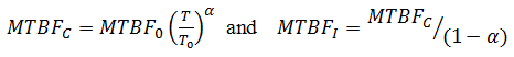 where “T” is the test time, “T0” is the time at the beginning of the monitoring period (initial time interval), “MTBFC” is the cumulative MTBF at time “T”, “MTBFI” is the instantaneous MTBF at time “T”, and “α” is the growth rate.
The Duane model is often used to plan a reliability growth test. For example, consider the data provided in Table 1 for a proposed RGT for a Signal Processing Computer.
Table 1: Sample Reliability Growth Test Parameters
| Parameter |
Symbol |
Value |
| MTBF Goal |
MTBFI |
2,000 |
| Initial MTBF (Average over 1st Test Phase) |
MTBF0 |
500 |
| Length of 1st Test Phase |
T0 |
1,000 |
| Growth Rate |
α |
0.35 |
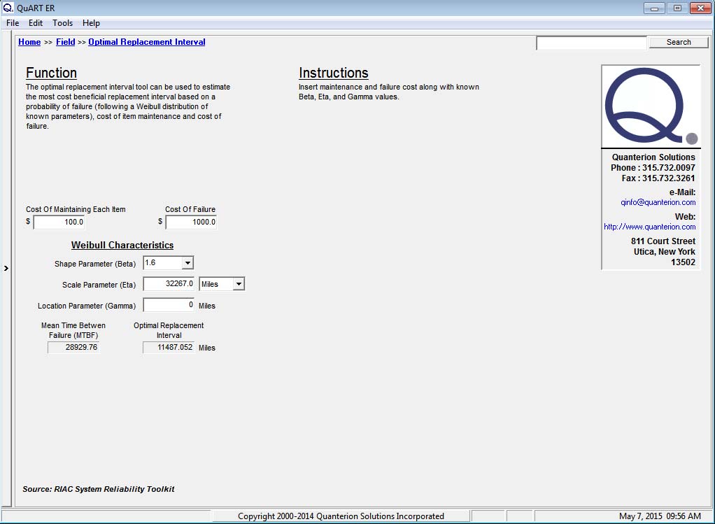
The test time necessary to grow the reliability from 500 to 2,000 hours can be calculated by substituting the values provided in Table 1 into the Duane model equations above and solving for “T”. In this example, the total required test time is 15,333 hours. If 4 test articles are used, then the total test time per article is 3,833 hours. The “Duane Method” calculator in the Quanterion Automated Reliability Toolkit – Enhanced Reliability (QuART-ER) (Figure 1) and QuART-PRO can be used to perform the calculations. If the required test time is prohibitive, then a more aggressive approach to precipitating and correcting failures should be considered, which could justify a higher growth rate.
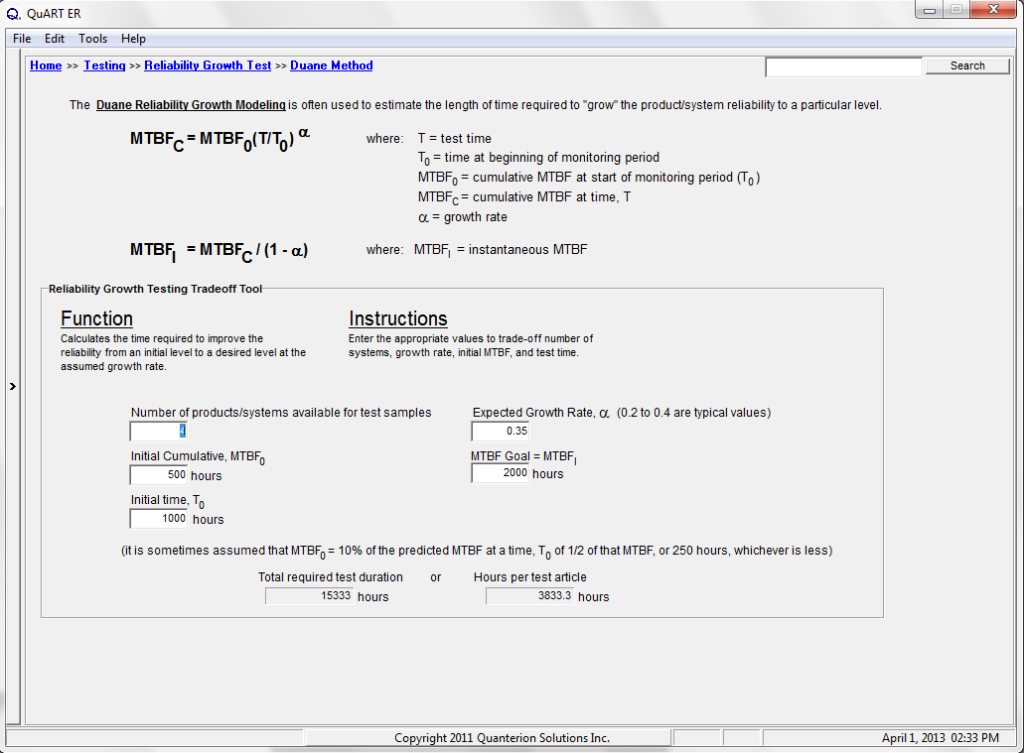
Figure 1: QuART-ER Duane Method Calculator
AMSAA-Crow Model
The AMSAA-Crow model, alternately referred to as the Reliability Growth Tracking Model Continuous (RGTMC) model, employs the Weibull process to track and model reliability growth during a development test phase. Growth within a test phase occurs when at least some corrective actions are incorporated as failures occur. The AMSAA-Crow model allows the engineer to estimate the instantaneous failure rate (and hence, MTBF) based upon a demonstrated cumulative failure rate pattern within a test phase. It assumes that failures within a test phase follow a non-homogeneous Poisson process, and that the instantaneous failure rate can be approximated with a Weibull intensity function described by shape parameter “beta” and scale parameter “lambda”. Mathematically, the AMSAA-Crow model can be represented by:
![]() where “ρ(t)” is the instantaneous failure rate at time “t”, “MTBFI” is the instantaneous MTBF at time “t”, “β” is the shape parameter, and “λ” is the scale parameter.
where “ρ(t)” is the instantaneous failure rate at time “t”, “MTBFI” is the instantaneous MTBF at time “t”, “β” is the shape parameter, and “λ” is the scale parameter.
“β < 1” implies that reliability growth is occurring (decreasing failure rate); “β > 1” implies that deterioration is occurring (increasing failure rate); and “β = 0” implies no growth (constant failure rate).
For example, consider the sample RGT data for the Signal Processing Computer shown in Table 2.
Table 2: Sample Reliability Growth Test Data
| Failure Number |
Test Article #1 |
Test Article #2 |
Test Article #3 |
Test Article #4 Hours |
Test Article #5 |
Cumulative Hours |
|
1 |
14.3* |
0 |
0 |
0 |
0 |
14.3 |
|
2 |
55.0* |
19.2 |
0 |
0 |
0 |
74.2 |
|
3 |
88.4 |
21.5* |
18.4 |
15.8 |
0 |
144.1 |
|
4 |
104.4* |
44.6 |
21.3 |
21.7 |
31.9 |
223.9 |
|
5 |
149.5 |
69.2 |
32.0* |
38.7 |
39.6 |
329.0 |
|
6 |
182.3 |
98.7* |
75.4 |
51.2 |
49.8 |
457.4 |
|
7 |
214.2 |
149.7 |
121.5 |
64.6* |
79.0 |
629.0 |
|
8 |
263.0 |
198.6 |
170.3 |
113.4 |
80.4* |
825.7 |
|
9 |
288.1* |
225.4 |
197.1 |
140.2 |
107.2 |
958.0 |
|
10 |
314.3 |
251.6 |
209.9* |
166.4 |
133.5 |
1075.7 |
|
11 |
381.8 |
262.6* |
277.3 |
233.9 |
200.9 |
1356.5 |
|
12 |
400.0 |
334.1 |
348.8 |
250.3* |
272.5 |
1605.7 |
|
13 |
400.0 |
382.2 |
396.9 |
298.3 |
293.0* |
1770.4 |
|
14 |
400.0 |
400.0 |
400.0 |
385.4* |
400.0 |
1985.4 |
|
END |
400.0 |
400.0 |
400.0 |
400.0 |
400.0 |
2000.0 |
*Indicates failure occurrence Calculating the AMSAA-Crow parameters at the end of the test (T = 2,000 hours), we have (where “F” is the total number of failures and “Xi” is the cumulative failure time of the “ith” failure):
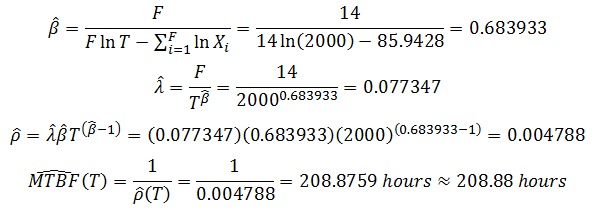 From these calculations, it can be concluded that reliability growth is occurring (“β < 1”), and that the instantaneous MTBF at the end of the test is approximately 209 hours.
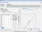
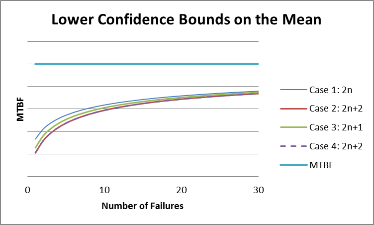
These calculations can also be performed using the QuART-ER AMSAA-Crow calculator as shown in Figure 2. QuART-ER also allows for a confidence interval to be constructed around the MTBF data, and it performs a goodness-of-fit test. As shown in Figure 2, the 80% confidence interval on the instantaneous MTBF is (126.16 hours, 385.58 hours) and the goodness-of-fit test indicates that the AMSAA-Crow model describes the failure data. (Note, the AMSAA-Crow calculator is not included in QuART-PRO.)
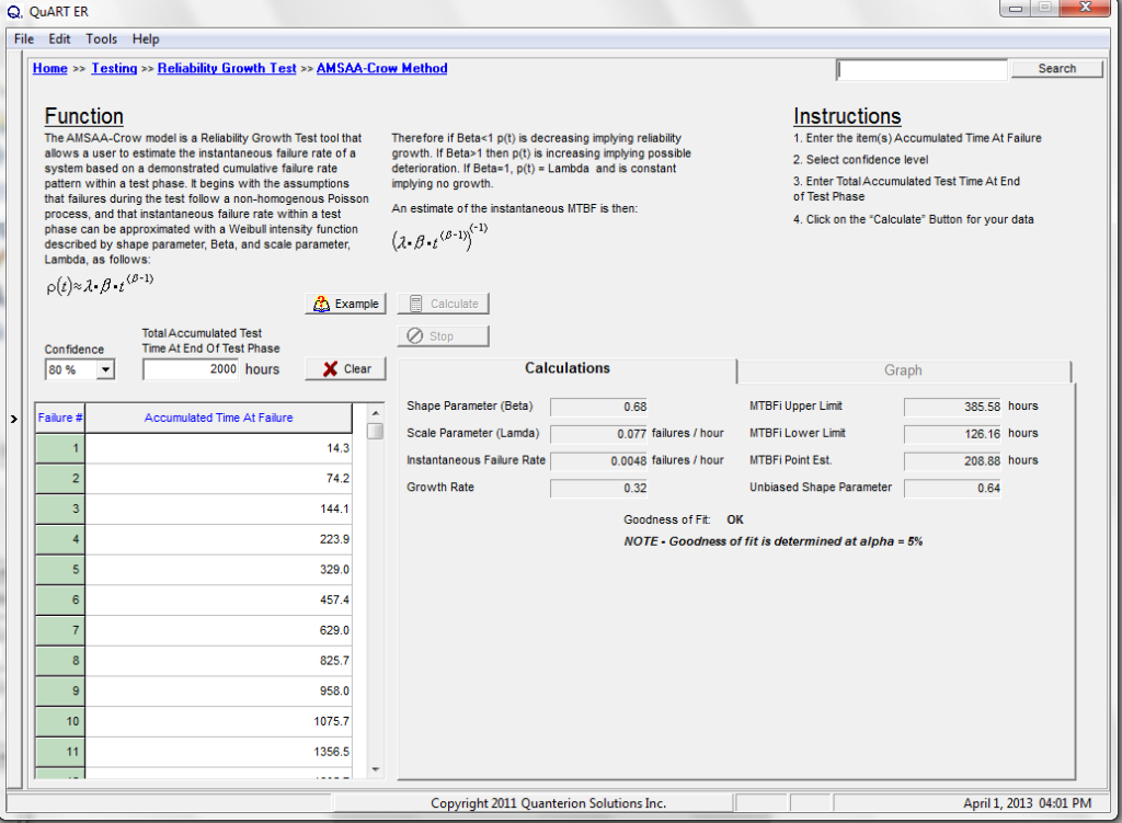
Figure 2: QuART-ER AMSAA-Crow Calculator
Crow Extended Model
The Extended Reliability Growth Projection Model for test-fix-find-test was developed by Crow and presented at the 2004 Reliability and Maintainability Symposium (RAMS) to address the common and practical case where some corrective actions are incorporated during test and some corrective actions are delayed and incorporated at the end of the test. In the application of the Crow Extended model, three types of failure modes are considered: “A” modes, which are those failure modes that will not receive corrective action; “BC” modes, which are those failure modes that will have corrective action incorporated during test; and “BD” modes, which are those failure modes whose corrective action is delayed until the end of the test (or test phase).
During test, the A- and BD-failure modes do not contribute to reliability growth. The corrective actions for the BC-modes influence the growth in the system reliability during the test. After the incorporation of corrective actions for the BD-modes at the end of the test, the reliability increases further, typically as a discrete jump. Estimating this increased reliability with test-fix-find-test data is the objective of the Crow Extended Model.
The Crow Extended Model also introduces the concept of “fix effectiveness”. Fix effectiveness is based upon the idea that corrective actions may not completely eliminate a failure mode and that some residual failure rate due a particular mode will remain. The “fix effectiveness factor” or “FEF” represents the fraction of a failure mode’s failure rate that will be mitigated by a corrective action. An FEF of 1.0 represents a “perfect” corrective action; while an FEF of 0 represents a completely ineffective corrective action. History has shown that typical FEFs range from 0.6 to 0.8 for hardware and higher for software.
As an example, the failure data presented in the previous example will now be categorized into specific failure modes and types as shown in Table 3.
Table 3: Sample Reliability Growth Test Data for Crow Extended Model
| Failure Number |
Cumulative Hours |
Failure Mode Number |
Failure Mode Type |
Fix Effectiveness |
|
1 |
14.3 |
1 |
BD |
0.7 |
|
2 |
74.2 |
2 |
BC |
N/A |
|
3 |
144.1 |
3 |
BC |
N/A |
|
4 |
223.9 |
1 |
BD |
0.7 |
|
5 |
329.0 |
1 |
BD |
0.7 |
|
6 |
457.4 |
4 |
BD |
0.8 |
|
7 |
629.0 |
5 |
A |
N/A |
|
8 |
825.7 |
1 |
BD |
0.7 |
|
9 |
958.0 |
1 |
BD |
0.7 |
|
10 |
1075.7 |
6 |
BC |
N/A |
|
11 |
1356.5 |
4 |
BD |
0.8 |
|
12 |
1605.7 |
1 |
BD |
0.7 |
|
13 |
1770.4 |
5 |
A |
N/A |
|
14 |
1985.4 |
7 |
BD |
0.75 |
|
END |
2000.0 |
As we can see, there are 7 unique failure modes including 1 A-mode, 3 BC modes and 3 BD modes. The first occurrence times of each of these modes are shown in Table 4.
Table 4: First Occurrence Times for Sample Reliability Growth Test Data
| Failure Mode |
First Occurrence |
Failure Mode |
Fix Effectiveness |
|
1 |
14.3 |
BD |
0.7 |
|
2 |
74.2 |
BC |
N/A |
|
3 |
144.1 |
BC |
N/A |
|
4 |
457.4 |
BD |
0.8 |
|
5 |
629.0 |
A |
N/A |
|
6 |
1075.7 |
BC |
N/A |
|
7 |
1985.4 |
BD |
0.75 |
Quanterion’s QuART-ER Crow Extended Model calculator can be used to calculate the projected MTBF at a given point in time. (The Crow Extended Model calculator is not included in QuART-PRO.) This process involves three steps. First, the seven unique failure modes are entered into Table 1 of the calculator as shown in Figure 3. The first occurrence times are entered into the “Failure Mode’ column; the mode type is entered into the “When Correcting” column (“Not Correcting” = A-mode, “In Test” = BC-mode, “After Test” = BD-mode); and the fix effectiveness is entered (in percent) for BD modes in the “Fix Effectivity” column.
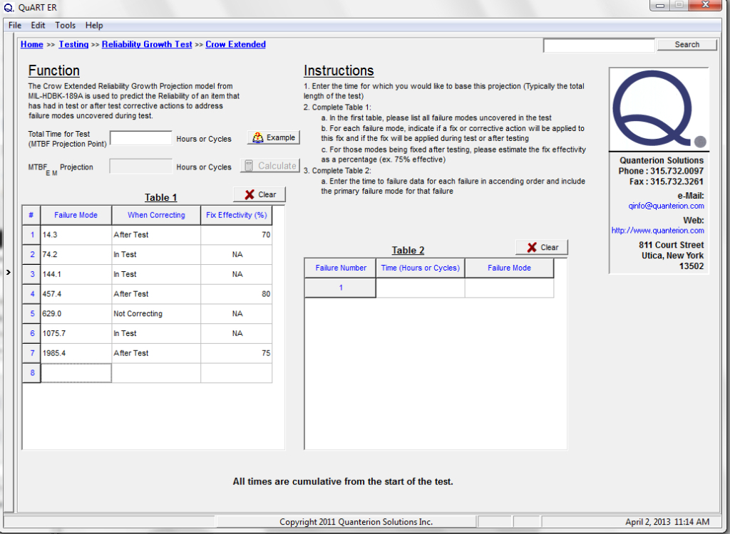
Figure 3: QuART-ER Crow Extended Calculator – Step 1
In the second step, the individual failures are entered into Table 2 of the calculator. The failure occurrence time is entered into the “Time” column, and the failure mode number to which the failure applies is entered into the “Failure Mode” column. In the final step, the total test time is entered into the appropriate field and the “Calculate” button is pressed. The projected MTBF is then displayed. The results of Steps 2 and 3 are shown in Figure 4.
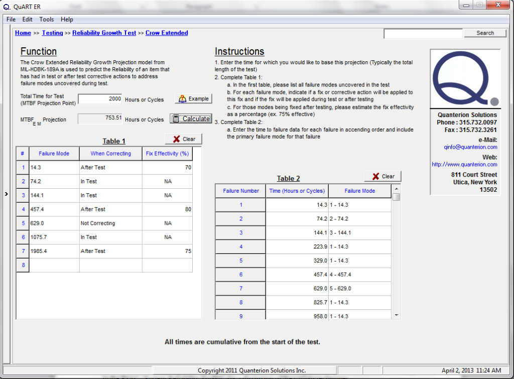
Figure 4: QuART-ER Crow Extended Calculator – Steps 2 and 3
As shown in Figure 4, the projected MTBF at 2000 hours is 753.51 hours. Using this calculator, projected MTBFs at various test times can easily be determined. Additionally, if projections show that the desired MTBF goal is not likely to be achieved, changes in management strategy (e.g., a decision to correct an A-mode) can be modeled by changing the mode type and including a fix effectiveness.
Summary
A brief overview of the Duane, AMSAA-Crow, and Crow-Extended methods of modeling reliability growth have been provided here, along with sample calculations using Quanterion’s QuART-ER calculator. A detailed discussion of reliability growth design and test methods, including these models, is presented in the RIAC’s “Achieving System Reliability Growth Through Robust Design and Test” publication and training program developed and offered by Quanterion. Additional information is also available on this topic through one of Quanterion’s RELease series of books titled “Reliability Growth“.