Design of Experiments for Reliability Improvement
Many times we want to improve Reliability (or other Quality characteristics) by way of increasing positive and reducing negative factor effects that influence performance.
For example, assume we want to increase the Mean Time Between Failures (MTBF) (or decrease the Mean Time To Reapir (MTTR)) of a product to improve its overall Availability. We need to first identify which factors are affecting the performance measure and then investigate what effects, if any, these factors have on it. By brainstorming, we can identify candidate factors that we can then put into a Fishbone chart. If our product is a vehicle, and we want to increase its MTBF, we may have:
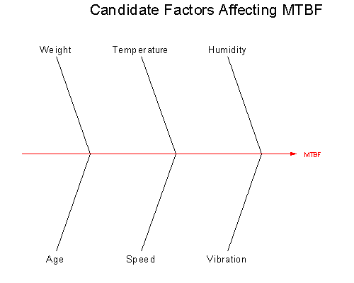
Figure 1 – Fishbone Diagram
We can assess the impact of the identified factors by implementing a Design of Experiments (DOE) approach and then analyzing the collected data. Often, however, the number of factors analyzed, which determine the number of test runs to implement, may make an experiment extremely costly or time consuming. We need to reduce the number of runs, in order to make it feasible. We can achieve this by implementing “Fractional” versions of Experimental Factorial Designs. Let’s work through an example.
Assume we are restricted to, at most, eight experimental runs. We select the four most important of the candidate factors, and carry out a four-factor Half Fraction Factorial DOE. We select Environmental Temperature (A), Humidity (B), Speed (C), and Weight (D). We use two conveniently selected levels for each factor: low (-) and high (+). This yields a ½ * ( 24 ) = ½ * 16 = 8 run Factorial design; one that we can now afford because we have reduced the number of runs from 16 (complete factorial) to only eight. Table 1 lists the most important factors and the low and high values for each factor.
Table 1 – Most Important Factors
| Factor | Low (-) | High (+) |
|---|---|---|
| Temp (°F) | 40 | 80 |
| Humidity (%) | 30 | 60 |
| Speed (MPH) | 30 | 50 |
| Weight (Tons) | 1 | 2 |
While there are many software tools available for DOE, we will use the Quanterion Automated Reliability Toolkit (QuART PRO). Enter MTBF as the Output Variable and the Factors and their values from Table 1 on the Problem Definition tab, as shown in Figure 2.
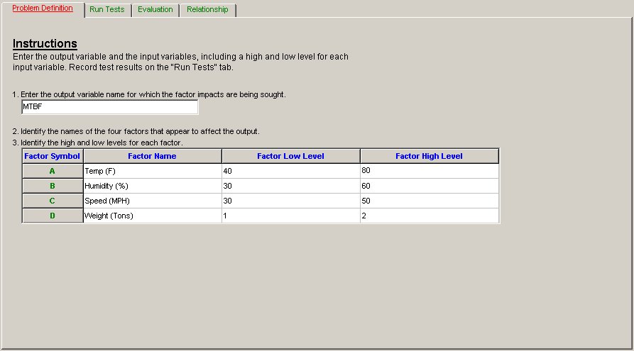
Figure 2 – Problem Definition Tab
The values for each Factor (e.g. Temperature, Humidity, etc.) are processed by the DOE algorithm in “coded” form. For each Factor, the two levels define a Range with a Minimum , a Midpoint, a Maximum, and a Half Range. For example, the Minimum for Temperature is 40°F which becomes -1 and the Maximum is 80°F which becomes +1. Its Midpoint is 60°F, and its Half Range is ½ the range, or 20°F (( 80 – 40 ) / 2). Any intermediate coded value is then interpolated between -1 and +1, using the formula:
| Coded = ( Real Value – Midpoint ) / Half Range | Eq. 1 |
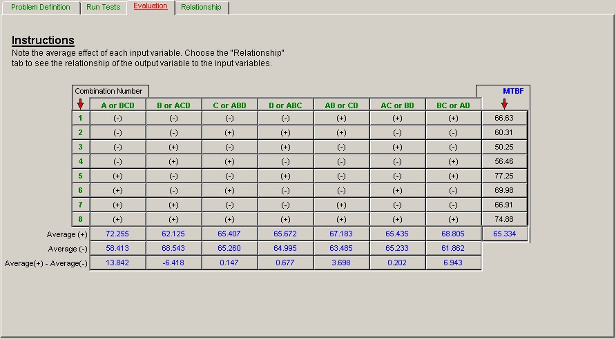
The experimental results, MTBF, of the implementation of the eight runs of the experiment are listed in Table 2 (letters A, B, C, D are used for Factor names and + and – for low and high levels, respectively).
Table 2 – Test Run Results
| Run | A | B | C | D | MTBF |
|---|---|---|---|---|---|
| 1 | – | – | – | – | 66.63 |
| 2 | – | – | + | + | 60.31 |
| 3 | – | + | – | + | 50.25 |
| 4 | – | + | + | – | 56.46 |
| 5 | + | – | – | + | 77.25 |
| 6 | + | – | + | – | 69.98 |
| 7 | + | + | – | – | 66.91 |
| 8 | + | + | + | + | 74.88 |
The MTBF results are entered on the Run Tests tab. It is crucial to be very carefully matching the run level combination with its corresponding MTBF result. For example, for the first run has the four lower levels of Temperature, Humidity, Speed, and Weight (i.e. 40°F, 30%, 30MPH and 1 Ton). The experimental MTBF was 66.63 hours. The Run Tests tab should look like Figure 3.
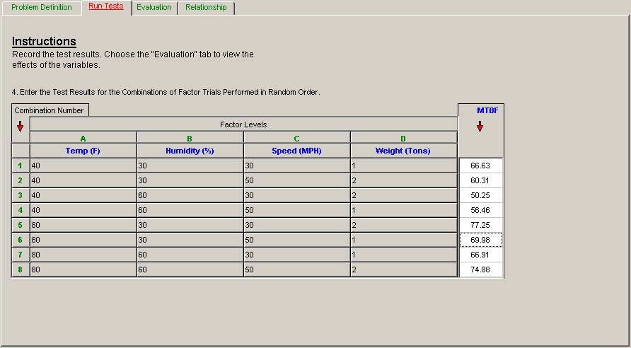
Figure 3 – Run Tests Tab
Once all the data is entered, select the Evaluation tab. There, the numerical results for our ½ * ( 24 ) = ½ * 16 = 8 run 1/2 Half Fractional Factorial are given. The Evaluation tab should look like Figure 4.

Figure 4 – Evaluation Tab
The key results of this tab are in the bottom line of the table, denoted “Average(+) – Average(-).” These are the “Main Effects” of each of the Factors (A, B, C, and D). These values constitute their (positive or negative) contribution to the response MTBF, as each Factor moves from the low to the high level. For example, Factor A has a positive effect (i.e., value 13.842) on the response MTBF.
There is, however, a price to pay when using a Half Fraction Design as opposed to a Full Design. When using the Half Fraction Design, the Factor Effects are “confounded”. That is, certain main effects and interactions are inextricably mixed so one cannot tell whether the “effect” is the Main Effect or an Interraction.
For example, Factor A in column 1, is “confounded” with Interaction “BCD”. Therefore, we cannot say whether this effect is due to A, or to BCD (or perhaps to both). However, higher order interactions are usually not very significant. Also, if there is prior knowledge about the vehicle under analysis, it can be used to resolve this issue. Therefore, confounding of effects is something that can usually be handled.
We still have to assess, statistically, the results obtained. Such assessment is found on the next tab, Relationship. The Relationship tab should look like Figure 5.
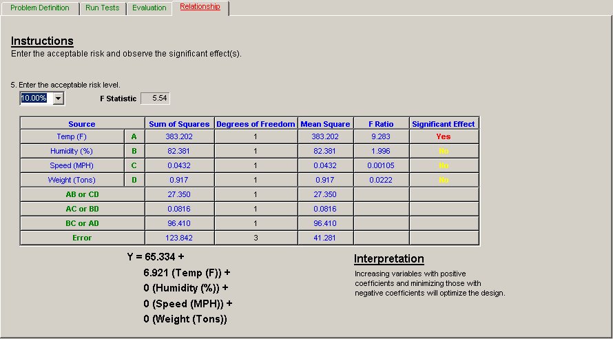
Figure 5 – Relationship Tab
Here, we enter the “acceptable risk”, often called alpha, that we are willing to accept. This is the risk of stating that a Factor is significant when it is not. In our case, we would like this risk to be 10%. For this value, QuART PRO provides the Fisher “F” percentile for the corresponding Degrees of Freedom (in this case, DF are 1 and 3). The percentile F(1, 3; α = 0.05) = 5.54 serves as comparison for the ratios of the corresponding Factor Mean Square and the Error Mean Square (given in the F-Ratio column of this sub-section).
For example, for Factor A (Temperature), the only significant one here, the Ratio:
| F = 383.202/41.281 = 9.283 | Eq.2 |
Hence, we can state, with 90% confidence, for this example that the Temperature Factor has a positive influence in extending the reliability (MTBF). The experiment performed showed that vehicles operate longer without experiencing failure when operating in higher temperatures (80°F) than when operating in lower temperatures (i.e. colder weather: 40°F).
For this example, the other three factors, Humidity, Speed, and Weight, do not seem to have a significant effect on reliability (MTBF). This is determined by observing that none of their F-Ratios is larger than percentile F(1, 3; α = 0.05) = 5.54. QuART PRO provides such assessment in the last column of Relationships tab, Significant Effects.
Finally, at the bottom of the Relationship tab, the Response equation for the Output Variable (MTBF) is displayed. In our example, the equation is:
| Y = 65.334 + 6.921 * Temperature + 0 * Humidity + 0 * Speed + 0 * Weight | Eq. 3 |
Remember, however, that the values for the Factors (here, Temperature, Humidity, etc.) were processed by the DOE in coded form and have to be entered in the resulting formula also in “coded” form. For our example:
| Coded-T = (Temp-60) / 20 ; Coded-H = (Hum-45) / 15 ; etc. | Eq. 4 |
The response equation provides a point estimate of MTBF, for a specific setting. If we want an estimate MTBF for vehicle operation in an environment where the temperature is 70°F with 50% humidity and the vehicle is running at 40MPH carrying 1.5 tons, we first convert these values to coded form:
| Coded-T = (70-60) / 20 ; Coded-H = (50-45) / 15 ; etc. | Eq. 5 |
Hence, we enter 0.5 for Temperature 70, 0.33 for Humidity 50,% and Zero for 40 mph and 1.5 Tons, respectively, in the model equation:
| MTBF | = | 65.334 + 6.921 * 0.5 + 0 * (0.33) + 0 * 0 + 0 * 0 | Eq. 6 | ||
| = | 65.334 + 6.921 * 0.5 = 68.79 hours |
The QuART PRO DOE analysis ends by providing an interpretation of this equation:
“Increasing variables with positive coefficients and minimizing those with negative coefficients will optimize the design”.
This means that “statistically significant” coefficients are placed in the equation, and “non-significant” coefficients, appear with value Zero (i.e. have no influence). This example provides three non-significant Factors: Humidity, Speed, and Weight, at 10% risk, and one significant Factor: Temperature (6.921)
Summarizing, QuART PRO can help reliability engineers analyze their experiments and use their statistical results to optimize (or improve) their design (or operation). Additional information is available on this topic through one of Quanterion’s RELease series of books titled “Design of Experiments“.